First mission#
Mubody main class is called Mission, you can import as follows (matplotlib and numpy are also imported for later use):
from mubody.mission import Mission
import matplotlib.pyplot as plt
import numpy as np
This class contains the main methods to generate orbits in L2 (the second lagrangian point) of the Earth-Sun system. To be able to use it, you first need to create an instance. The Mission class and its methods have default values that allow to generate orbits directly. To calculate an orbit based on the analytic solution of the CRTBP:
upm = Mission()

upm.AO()

fig_tra = upm.plot_trajectory()

plt.show()

Once the orbit has been generated, the trayectory data (the state vector, position and velocity) is stored automatically inside the class in a dataframe structure which can be retrieved and converted to a numpy array. The index of the dataframe is the time corresponding to each state. Note that the resulting array will have table format, so each column is a variable. All the data is in the International System of Units and the default reference system is SEML2Synodic, i.e., the rotating system centered in the Sun-Earth/Moon system L2 point. This can be checked through the Mission class attribute “frame”. The time elapsed can be also extracted from the dataframe in a numpy array:
example_trajectory_df = upm.sat.orbit.tra_df
example_trajectory_array = example_trajectory_df.values
time = example_trajectory_df.index.values

print(upm.frame)
SEML2Synodic
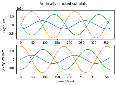
The position and the velocity can be interpolated for any instant whithin the simulation period using class methods
#interval instants for one year (seconds)
t1 = 0*86400
t2 = 365*86400

# interpolation instants
time_interest = np.linspace(t1,t2,100)

# for plotting
time_interest_days = time_interest/86400

r = upm.sat.r(time_interest)

v = upm.sat.v(time_interest)

fig, axs = plt.subplots(2)
fig.suptitle('Vertically stacked subplots')

axs[0].plot(time_interest_days, r.T)
axs[1].plot(time_interest_days, v.T)

axs[0].set(ylabel='(x,y,z) (m)')
axs[1].set(ylabel='(vx,vy,vz) (m/s)')
axs[1].set(xlabel='Time (days)')

plt.show()